Polynomials and Synthetic Divison

In this post, I want to talk about synthetic polynomial division and why the final value you get is BOTH the $y$ value of the function at a particular point AND the remainder when you perform the division. We’ll use one running example with coefficients $a_i$ , and even though our example will be with a cubic polynomial, the same idea generalizes to polynomials of any degree.

Let’s let $f(x) = a_3x^3+a_2x^2+a_1x+a_0$ , and lets let $g(x)=x-c$ . We want to compute $\frac{f(x)}{g(x)}$ . To do this, we’ll set up synthetic divison as follows.

Inside the box, we put the value that makes the denominator zero. One of the assumptions of synthetic division is that the highest degree on the $x$ term is $1$ . So, if $c$ is inside the box, we know that we are dividing by $x-c$ .

To the right of the box, we put the coefficients of the polynomial in question (in decreasing order of exponent). If there were a term missing as the powers decreased (like if the polynomial were $x^2+1$ (no $x$ term)), we would put a zero in that position.

Now, let’s do some synthetic division. This is a combination of two steps: add and multiply. In the first step, we’ll just be bringing down the first constant, but that’s the same as adding zero to the first constant. Here’s the result if you carry out the synthetic division in this example.

The last term in the last column above the horizontal line that’s hard to read is $c^3a_3$ .

The expression in last column of synthetic division below the blue line always gives the remainder of the polynomial division. However, we can ALSO see that this expression $(a_0+ca_1+c^2a_2+c^3a_3)$ is the same as $f(c)$ , or the function $f$ evaluated at $x=c$ .

Hang on, that’s pretty cool. The remainder of the polynomial division by $(x-c)$ is the same as $y-$ value of the function at $x=c$ .

Now let’s talk about why the final term being zero when plugging in $c$ corresponds to $(x-c)$ being a factor of $f(x)$ . If $f(c)=0$ , then we can write $f(x)$ as a product of two polynomials, $f(x)=(x-c)\cdot h(x)$ , where $h(x)$ is some other polynomial (Note that if you evaluate $f(c)$ , you’ll get $(c-c)\cdot h(c)=0\cdot h(c)=0$ ).

Even if the term you’re dividing by is not a factor of $f(x)$ , we see that synthetic division still gives you the $y-$value at that point. Thinking in terms of remainders, this also makes a lot of sense. The remainder after division can be thought of as a measure of how far the denominator was from being a factor of the numerator. If, at $x=a$ , the $y-$ value of the function was $4$ , then the numerator was $4$ more than a multiple of the denominator. In other words, if you subtract $4$ from the numerator, it will be divisible by the denominator with no remainder. And, this will have created a polynomial which IS a multiple of the denominator.

Let’s look at an example to make this a little more concrete. Let’s let $f(x)=x^3-1$ , and let’s let $g(x)=x-2$ . Then, the synthetic division will look like this.

The final value in the bottom right is $7$, so this should be the $y-$value of the function at $x=2$ . We can check that $f(2)=2^3-1=7$ . Also, if the remainder is $7$ , then we should be able to subtract $7$ and obtain a multiple of $(x-2)$ . Let’s see if that works.

$x^3-1-7=x^3-8=(x-2)(x^2+2x+4)$ . Indeed, $(x-2)$ is a factor of that new polynomial!

I hope this helped you see a connection between zeros and factors of polynomials! And how the output of synthetic division relates to the numerator function’s value at a particular point!

Remember to post this on Facebook and tell your friends about it! Also, you can subscribe to posts so you can be the first to read the next one!

Rational Root Theorem

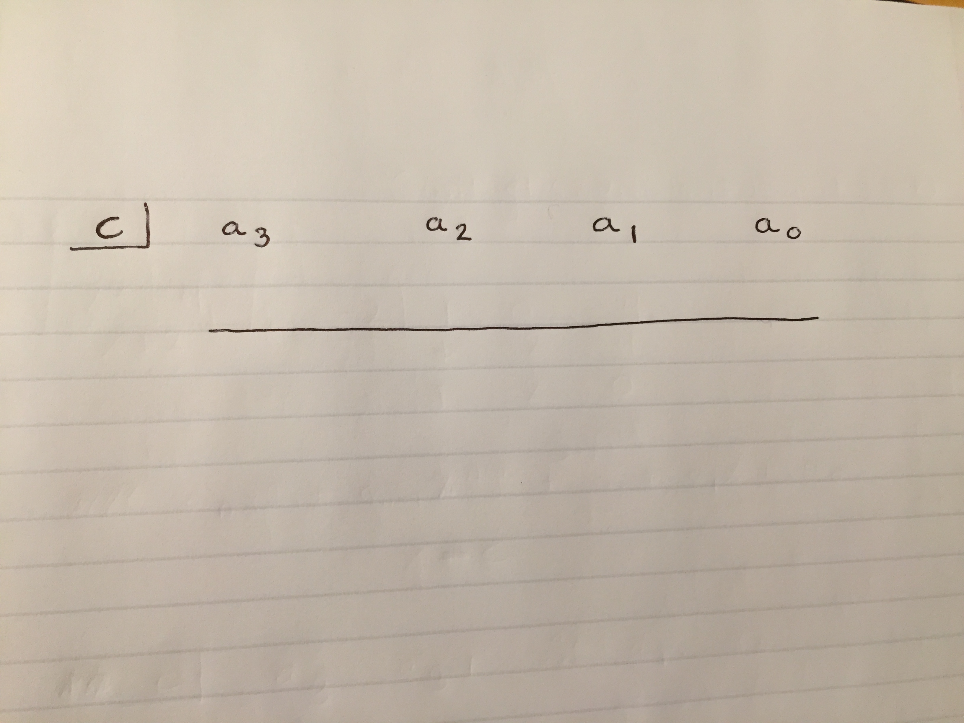
This post is a follow-up to the last post about the Fundamental Theorem of Algebra. As a recap, the Fundamental Theorem of Algebra says that if you have a polynomial of degree $n$ with coefficients in $\mathbb{C}$ , then the polynomial will have $n$ roots in $\mathbb{C}$ .

As we talked about last time, the Fundamental Theorem of Algebra is an existence proof because for a polynomial of degree $n$ whose coefficients are in $\mathbb{C}$ , it says that you’ll be able to find $n$ values which, when plugged into the polynomial, make the polynomial equal zero. In other words, you’re guaranteeing the existence of the values that will make the polynomial equal zero.

Existence proofs are cool and all, but the Fundamental Theorem of Algebra doesn’t tell us anything about how to find the $x-$ values that make the polynomial equal zero. Wouldn’t it be nice if there were a way to know where these zeros were?

It turns out that if we restrict ourselves to looking for rational zeros of a polynomial, then we can say exactly what those kinds of zeros would have to look like. Now, let’s state the Rational Root Theorem.

Rational Root Theorem: If a polynomial $f(x) = d_0x^n+d_1x^{n-1}+\ldots+d_{n-1}x+d_n$ has any rational zeros, then they will have to occur at $x=\frac{p}{q}$ , where $\pm p$ is some factor of $d_n$ and $\pm q$ is some factor of $d_0$ .

To prove the Rational Root Theorem, we’re going to write a polynomial as a product of terms, which the Fundamental Theorem of Algebra guarantees we can do.

Proof: Let $f(x) = (a_1+b_1x)(a_2+b_2x)\ldots(a_n+b_nx)$ , where the “ $\ldots$ ” includes the product of other linear terms. First, let’s find the zeros of this function. To do that, we want to solve $(a_1+b_1x)(a_2+b_2x)\ldots(a_n+b_nx) = 0$ . Note that we won’t always be able to get $n$ factors multiplied together if there are some factors that don’t yield rational roots. But even if you can’t, that gives you information, too! For example, there might be a polynomial with five roots, only three of which are rational.

Before we solve for the values of $x$ that make this function equal zero, let’s just think about what the highest degree term and lowest degree term will look like. We don’t need to think about the terms that have degree $0<k<n$ . The highest degree term comes from multiplying all of the terms that have an $x$ in them. And the lowest degree term comes from multiplying all of the terms that are just constants. This means that the highest degree term will be $(b_1)(b_2)\ldots (b_n)x^n$ . And the lowest degree term will be $(a_1)(a_2)\ldots (a_n)$ .

Let’s remember that we’re trying to solve $(a_1+b_1x)(a_2+b_2x)\ldots(a_n+b_nx) = 0$ . Since the left-hand side is a product of $n$ terms that equals zero, the whole left-hand side will equal zero when any of these terms individually equals zero. So, this function has zeros when $x\in\{-\frac{a_1}{b_1},-\frac{a_2}{b_2},\ldots,-\frac{a_n}{b_n}\}$ .

Okay, we’re so close! We know that if our function has a rational zero, it will definitely be in the set $A=\{-\frac{a_1}{b_1},-\frac{a_2}{b_2},\ldots,-\frac{a_n}{b_n}\}$ , even though not all of these quotients have to be rational. And if we want to find these values, we just have to search the set of quotients $\{\frac{p_i}{q_i}\}$ , where $p_i$ is a factor of $a_1a_2\ldots a_n$ and $q_i$ is a factor of $b_1b_2\ldots b_n$ because that will check all of the values in $A$ , which is the set of all zeros.

This theorem says that IF a function has rational zeros, then here’s how to find them. But there’s no guarantee that a function will have rational zeros to begin with.

So, to recap: The Fundamental Theorem of Algebra states the existence of $n$ complex-valued zeros for a polynomial of degree $n$ , but is kind of like “good luck!” when it comes to actually finding these zeros. Then the Rational Root Theorem comes along and says, “hey, if you don’t mind only looking for rational zeros of this function, I can help you out!” It says that any rational root of your polynomial can be written as the quotient of two integers, where the numerator is a factor of the constant term and the denominator is a factor of the highest degree term.

I hope this helped you see a connection between the Fundamental Theorem of Algebra and the Rational Root Theorem!

Remember to pass this page along to your friends and ask them to share it!

Fundamental Theorem of Algebra

In this post, I want to talk about the Fundamental Theorem of Algebra. Really, this could be called “Why the Complex Numbers are Cool.” For a while, I don’t really think I appreciated what this theorem was saying, but now I think I have a better way to think about it. Let’s start by stating the Fundamental Theorem of Algebra.

Theorem: Every polynomial with coefficients in $\mathbb{C}$ of degree $n$ has exactly $n$ roots in $\mathbb{C}$ .

Let’s look at an example to see this in action.

Example: Consider the polynomial $f(x) = x^3+x^2+x+1$ . This polynomial equals zero in three places (when $x=i, x=-i,x=-1$ ). This definitely satisfies the theorem because $f(x)$ has degree $3$ . (Remember that the degree of a polynomial refers to the power of the highest degree term.)

To get an appreciation for why this theorem is REALLY about the complex numbers as a field, let’s look at an example of a polynomial that has coefficients in a different field.

We’ll do an example using the field $\mathbb{Z}_3$ . First, we can note that $\mathbb{Z}_3$ is a ring because we can define addition and multiplication on it and the set is closed under both of these operations. Also, it has an additive identity and multiplicative identity and every element has an additive inverse. This ring is also a field because every non zero element has a multiplicative inverse that is also in the set. We can see this since $1^2 = 1$ and $2^2 = 4$ mod $3 \equiv 1$ . So, in $\mathbb{Z}_3$ , every nonzero element is its own inverse! Kind of cool! Now, let’s look at a polynomial with coefficients in $\mathbb{Z}_3$

Example: Consider the polynomial $g(x)=x^2+1$ , where we consider the coefficients of $g(x)$ as being elements of $\mathbb{Z}_3$ . Now, in searching for zeros of this function, we’re restricted to looking at values that are in $\mathbb{Z}_3$ . This isn’t that hard to do since there are only three values to check.

$g(0) = (0^2+1)$ mod $3 \equiv 1$ .
$g(1) = (1^2+1)$ mod $3 \equiv 2$ .
$g(2) = (2^2+1)$ mod $3 \equiv 2$ .

We take each output mod $3$ because we are in the field $\mathbb{Z}_3$ .

So after building a polynomial with coefficients in $\mathbb{Z}_3$ , it has no zeros in $\mathbb{Z}_3$ . This shows that the complex numbers are really special as far as fields go! In fact, here’s another way that the Fundamental Theorem of Algebra is sometimes stated.

Theorem: The field of complex numbers is algebraically closed.

We can’t say this about $\mathbb{Z}_3$ since we built a polynomial with coefficients from that field that doesn’t have zeros in that field.

The last thing I want to say about the Fundamental Theorem of Algebra is that it’s an existence proof! Existence proofs show up all over different areas of math (analysis, number theory,…other places (?)). Why is this an existence proof? Because for any degree $n$ polynomial with coefficients in $\mathbb{C}$ , the theorem claims that THERE EXIST $n$ values in $\mathbb{C}$ that make this polynomial equal zero.

I hope this helped you care a little bit more about the Fundamental Theorem of Algebra and that you love the complex numbers just a little bit more than you did before (who thought that was even possible? Not me, for sure!).

A Nice Distribution on the Real Numbers

I wanted to call this post “Throwing Darts at the Real Numbers,” but apparently someone else already came up with that title to talk about something else. This is a follow-up to the last post that talked about why it’s not possible to define a uniform distribution on an unbounded set (like $\mathbb{Z}$ or $\mathbb{R}$ ).

Even though it’s not possible to uniformly sample from the real numbers, is there something else that we can choose uniformly that will induce a certain distribution on the real numbers? There is!

What if we were standing some fixed distance (say, $1$ unit) away from the real numbers and threw darts at it? If we throw darts at the real numbers, we can describe our throw by the angle that the dart’s path makes with the real number line.

The red line describes the path of the dart towards the real number line, and the angle $\theta$ describes the angle that the dart’s path makes with the line.

Suppose if you were to draw a perpendicular line through where you were standing to the number line, that it passed through the value $0\in \mathbb{R}$ (slide over the stick figure a bit to the right).

Now, we can define a nice distribution on $\mathbb{R}$ by picking angles $\theta\in [-\frac{\pi}{2},\frac{\pi}{2}]$ uniformly from the probability density function (PDF) $\theta \sim U[-\frac{\pi}{2},\frac{\pi}{2}]$ . This PDF has the equation $f(x)=\frac{1}{\pi}$ when $x\in [-\frac{\pi}{2},\frac{\pi}{2}]$ and $f(x)=0$ when $x<-\frac{\pi}{2}$ or $x>\frac{\pi}{2}$ . This means that, for example, picking an angle between $-\frac{\pi}{4}$ and $\frac{\pi}{4}$ is just as likely as picking an angle between $0$ and $\frac{\pi}{2}$ .

Let’s say you are standing 1 unit away from the real number line and in line with 0 and compute the probability that the dart you throw hits somewhere between 1 and 2.

To compute this probability, we need to find the angle between where you’re standing and each of those points on the number line. Here are the pictures to have in your head.

Now, we want to find the upper and lower bounds of $\theta$ that create these the triangles with top side lengths between 1 and 2. We’re measuring these angles in radians, but it doesn’t really matter as long as we divide by the appropriate scaling factor.

In the first triangle, $\theta=arctan(\frac{1}{1})=\frac{\pi}{4}\approx 0.7854$ , and in the second triangle, $\theta=arctan(\frac{2}{1})\approx 1.107$ .

Now we can compute the probability of hitting this region as $\frac{arctan(1)-arctan(2)}{\pi}\approx 0.1024$ . There’s a $\pi$ in the denominator since from all the way parallel to the number line facing to the left and all the way parallel to the number line facing to the right makes up $\pi$ radians.

This means that if you pick angles uniformly between $-\frac{\pi}{2}$ and $\frac{\pi}{2}$ , there is roughly a 10.24% chance that the number you hit will be in between 1 and 2.

Isn’t that kind of cool? I think so. I’m not sure if this is a standard distribution, so if anyone has any insight into that, let me know!

Probability is Strange: Example 1

Really, this is just Part 2 of Why The Real Numbers are Cool (name adapted). Let’s start by stating a strange fact.

There is no way to uniformly sample values from an unbounded set (like $\mathbb{R} \text{ or } \mathbb{Z} \text{ or } \mathbb{N}$ ). To get an appreciation for this, let’s first define the uniform probability distribution.

Definition: A continuous probability distribution is uniform if its probability density function is given by $f(x)=\frac{1}{b-a}$ , when $a\leq x\leq b$ and $f(x)=0$ when $x< a$ or $x>b$ .

Definition: A discrete probability distribution is uniform if its probability mass function is given by $\mathbb{P}(X=x)=\frac{1}{n}$ .

We’ll first prove that there is no continuous uniform probability density function on an unbounded set, which we’ll do by contradiction.

Suppose that we could define a uniform probability distribution over $\mathbb{R}$ . This function $f(x)$ would have to satisfy $\int_{-\infty}^{\infty} f(x) dx = 1$ . Since we are supposing that $f(x)$ is constant, we could rewrite this as $\int_{-\infty}^{\infty} c dx = 1$ . The region over which we’d like to integrate has an infinitely long bottom side (given by the integration bounds). Since the height should be the same everywhere, any infinitely long rectangle (no matter how short), will have an infinite area.

This means that we won’t be able to define a function that is constant over all of $\mathbb{R}$ and integrates to 1. So, any probability density function over $\mathbb{R}$ will have to assign a higher probability to some regions than others. We specify regions because for continuous probability density functions, there’s no notion of the probability that a random variable is equal to a certain value (only that it is in the range of particular values).

In the discrete case, let’s try to define a uniform probability mass function over $\mathbb{N}$ . Since every integer should be equally likely, this would mean that for any $n\in\mathbb{N}$ , $\mathbb{P}(X=n)=k$ , for some $k\in\mathbb{R}$ . Since there are infinitely many natural numbers, we would have to be able to evaluate $k+k+\ldots = 1$ . But, no matter how small $k$ is, this sum will always grow without bound!

This means that we won’t be able to assign an equal probability to every element in $\mathbb{N}$

The thing that’s so strange about this is that when someone asks you to pick a random positive integer, even if you think you’re being totally unbiased, you are never giving every number an equal chance of being picked.

The real numbers were used as an example for a continuous random variable, but any continuous-valued random variable will have the same problem. Similarly, just because we showed an example with the natural numbers, you’ll have the same problem if you use the integers or some other countably infinite set.

What’s interesting about this is that it kind of shows how even if you try to choose integers or real numbers in a way is consistent with intuition (like choosing which chair to sit in), it’s not possible!

The Nested Interval Property

In this post, I want to talk about the definition of completeness, and then use the completeness of the real numbers to prove the Nested Interval Property. Before we define completeness, we need the definition of a Cauchy sequence.

Definition: A sequence $\{x_1,x_2,\ldots,x_k,\ldots\}$ of real numbers is called Cauchy if for all $\epsilon>0$ , there exists an $N\in\mathbb{N}$ such that for all natural numbers $m,n>N$ , $|x_m-x_n|<\epsilon$ .

This definition says that a sequence is Cauchy if, for any positive tolerance (no matter how small), you can go far enough out in the sequence (past $N$ ) where any two elements past that certain point will be closer together than the tolerance you chose.

A good intuition for this definition is that, in a Cauchy sequence, all of the terms of the sequence get arbitrarily close together eventually (after some a given point). The point after which this happens depends on the tolerance you set (how close together you want all of the elements to be).

Now, let’s define what it means for a space to be complete.

Definition: A metric space $\mathbb{M}$ (for example, $(\mathbb{R},|\cdot|)$ ) is complete if every Cauchy sequence with elements in $\mathbb{M}$ converges to an element in $\mathbb{M}$ .

What this definition is really saying is that a space is complete if, whenever all of the terms are getting arbitrarily close to each other, they are also getting arbitrarily close to an element of the space that they’re in.

Now let’s talk about the Nested Interval Property. This is a statement about the real numbers that says…

Let $\{I_1,I_2,\ldots\}$ is a sequence of nested closed intervals, which look something like this:

Adapted from https://en.wikipedia.org/wiki/Nested_intervals

Then the infinite intersection $\bigcap_{n=1}^{\infty} [A_n,B_n]$ is non-empty. This property says that no matter how close you zoom in on the real number line, there will always be real numbers where you are looking.

Now, let’s use the completeness of the real numbers to prove the Nested Interval Property.

When we build the sequence of nested intervals $\{[A_1,B_1],[A_2,B_2],\ldots\}$ , we’re simultaneously constructing two sequences of real numbers: One increasing sequence $\{A_1,A_2,\ldots,\}$ , and one decreasing sequence $\{B_1,B_2,\ldots\}$ .

These sequences will definitely be Cauchy because the upper limit of the increasing lower bounds can never exceed the lower limit of the decreasing upper bounds. (i.e., $sup\{A_n\}\leq inf\{B_n\}$ ).

Since every Cauchy sequence converges, we know that both of these sequences will converge. And this guarantees that the infinite intersection $\cap_{n=1}^{\infty} I_n$ of the nested sets will be nonempty!

First Isomorphism Theorem Example

In this post, I want to talk about an application of the First Isomorphism Theorem to linear transformations between different dimensions. We’ll see why it’s kind of surprising why this works at all, but also why it makes sense that it works.

Let’s start by stating the version of the First Isomorphism Theorem that we’ll be talking about.

First Isomorphism Theorem for Groups: Let $\phi: G\to H$ be a surjective homomorphism. Then $H$ is isomorphic to $G/ker(\phi)$ .

Note that since $\phi$ is surjective (onto), we can just say $H$ instead of $im(\phi)$ , since every element of $H$ gets mapped to by $\phi$ .

Example: Consider the transformation $y =\begin{pmatrix}1&0&0\\0&1&0\end{pmatrix}\begin{pmatrix}x_1\\x_2\\x_3\end{pmatrix}=\begin{pmatrix}x_1\\x_2\end{pmatrix}$ .

To apply the First Isomorphism Theorem to this example, we let $\phi$ be this linear transformation, where the group composition law is vector addition, satisfying $\phi(a+b)=\phi(a)+\phi(b)$ .

The kernel of this linear transformation is a vector of the form $\begin{pmatrix}0\\0\\k\end{pmatrix},$ for any $k\in\mathbb{R}$ .

Since this transformation goes from $\mathbb{R}^3$ to $\mathbb{R}^2$ , to examine $G/ker(\phi)$ , we need to figure out what $\mathbb{R}^3/ \begin{pmatrix}0\\0\\k\end{pmatrix}$ looks like. This is like asking, “what does everything in $\mathbb{R}^3$ that has a zero in the third position look like?”

This means that we can write $G/ker(\phi)$ as span{ $\begin{pmatrix}1\\0\\0\end{pmatrix},\begin{pmatrix}0\\1\\0\end{pmatrix}$ }.

The First Isomorphism Theorem says that this should be isomorphic to $\mathbb{R}^2$ . This makes a lot of sense, because the vectors in the set above are the $x$ and $y$ unit vectors (so they definitely span $\mathbb{R}^2$ ). Even though the result of taking the quotient group above lives in $\mathbb{R}^3$ , the only thing that this theorem cares about is the fact that the resulting set after taking the quotient is a two-dimensional plane.

Rank-Nullity Theorem and First Isomorphism Theorem

In this post, I want to talk about the connection between the Rank-Nullity Theorem from Linear Algebra and the First Isomorphism Theorem, which comes up in Abstract Algebra. We talked about the Rank-Nullity Theorem in the last post, but here’s a quick overview.

The Rank-Nullity theorem relates the dimension of the column space of an $m\times n$ matrix $A$ to the dimension of the null space of that matrix. Specifically, it says that the sum of these two values is equal to the number of columns of $A$ . That is, $rank(A)+nul(A) = n$ .

Before we talk about the First Isomorphism Theorem and relate it to linear transformations, let’s just define a few things that we’ll need to know to understand it.

Definition 1: The kernel of a transformation $f:A\to B$ is the set $\{x\in A \vert f(x)=0 \}$ . Note that $0\in B$ .

Note that the kernel is a generalization of the null space of a matrix that is defined for both linear and nonlinear transformations.

Definition 2: An element $b$ is in the image of a transformation $f:A\to B$ if there exists some $a\in A$ such that $f(a)=b$ .

The image of a transformation is a generalization of the column space that holds for both linear and nonlinear transformations. That is, the image of matrix transformation is the column space of that matrix.

Definition 3: A group homomorphism from $(G,*)$ to $(H,\cdot)$ is a function $h:G\to H$ such that for all $u$ and $v$ in $G$ , it holds that $h(u*v) = h(u)\cdot h(v)$

A good way to think about a group homomorphism is that it’s a transformation between groups that maintains the relationship between the groups elements. You will get the same result if you multiply two elements in $G$ and apply the function $h$ as if you apply the function $h$ to them both separately and then multiply the two outputs in the group $H$ together. This is interesting because the group composition rules are not necessarily the same.

Now, let’s state the specific case of First Isomorphism Theorem we’ll talk about.

First Isomorphism Theorem: Let $\phi:G\to H$ be a surjective homomorphism. Then, $H$ is isomorphic to $G/ker(\phi)$ . Since $\phi$ is surjective, $H=im(\phi)$ .

Hold on…What’s does $G/ker(\phi)$ mean? That notation is a quotient group. There is a formal definition of it, but for now, let’s think about it as a way to separate elements in $G$ into classes (called cosets) depending on their relationship with $ker(\phi)$ . This quotient group will have two cosets: one containing everything in $G$ that IS IN $ker(\phi)$ and one containing everything in $G$ that IS NOT IN $ker(\phi)$ .

Because of the way quotient groups work, if $\phi$ goes between spaces of the same dimension, the original group $G$ can be written as the union of two sets: $G = ker(\phi) \cup im(\phi)$ .

Since $G$ can be written in this way, it must be true that the size of $G$ is equal to the sum of the sizes of $ker(\phi)$ and $im(\phi)$ .

What does this say about linear transformations represented by square matrices? Since you can’t both be in a set AND not be in a set, it says that for a linear transformation from $\mathbb{R}^n$ to $\mathbb{R}^n$ , the null space and column space must be disjoint (except they’ll both have the zero vector in them).

Let’s look at a few examples and see why this makes sense.

Example: Let $C$ be an $n \times n$ invertible matrix. This means that the columns map onto $\mathbb{R}^n$ and also that the null space has only the zero vector, meaning that these two sets share only the zero vector.

Example: Consider the non-invertible matrix $\begin{pmatrix}1&2\\2&4\end{pmatrix}$ , which has the vector $\begin{pmatrix} 2 \\ -1 \end{pmatrix}$ in its null space. If you try to solve $\begin{pmatrix}1&2\\2&4\end{pmatrix}\begin{pmatrix}x\\y\end{pmatrix}=\begin{pmatrix}2\\-1\end{pmatrix}$ , you won’t be able to!

So, what have we learned? The First Isomorphism Theorem generalizes the Rank-Nullity Theorem in a way that lets us handle transformations between groups that are not necessarily Euclidean spaces. There is a tradeoff between having elements in the kernel of a transformation and elements in the image of a transformation. The larger the kernel is, the smaller the image is, and vice versa.

Let’s talk about the progression of these three theorems. The Invertible Matrix Theorem draws connections between the algebraic properties of a square matrix to the geometry of the transformation it represents. The Rank-Nullity theorem makes claims about the geometry of transformations between Euclidean spaces with potentially different dimensions. And the First Isomorphism Theorem makes claims about transformations between groups in general (note that $\mathbb{R}^n$ and $\mathbb{R}^m$ are groups for any integers $n$ and $m$ ).

In the next post, we’ll talk more about what the First Isomorphism Theorem is actually saying and a neat application of it to transformations between different dimensions.

Stay tuned!

Invertible Matrix Theorem and Rank-Nullity Theorem

Let’s talk about a way to connect two theorems that come up in Linear Algebra: the Invertible Matrix Theorem (IVT) and the Rank-Nullity Theorem.

The Invertible Matrix Theorem has a lot of equivalent statements of it, but let’s just talk about two of them. Here’s the first one.

$\bf{Definition}$ : An $n\times n$ matrix $A$ is invertible if and only if $A\vec{x} = 0$ has only the solution $\vec{x} = 0$ .

Another way of saying this is that the null space is zero-dimensional. Usually, when a set is written as the span of one vector, it’s one dimensional. But in this case, since no scalar multiple of the zero vector actually scales it at all, the null space is zero-dimensional. We’ll use this fact when we talk about the Rank-Nullity Theorem.

Here’s another statement of the Invertible Matrix Theorem.

$\bf{Definition}$ : An $n\times n$ matrix $A$ is invertible if and only if its columns map onto $\mathbb{R}^n$

We are going to use these two characterizations of the Invertible Matrix Theorem to connect it to the Rank-Nullity Theorem. First, let’s define the rank and nullity of a matrix.

$\bf{Definition}$ : The rank of a matrix is the dimension of the column space of the matrix.

Since the column space lives in $\mathbb{R}^m$ , the rank of a matrix is less than or equal to $m$ .

$\bf{Example}$ : The matrix $A = \begin{pmatrix}1 & 0 \\ 0 &0 \\ 0&0 \end{pmatrix}$ has rank $1$ , since any vector in the column space is of the form $\begin{pmatrix}k \\ 0\\ 0 \end{pmatrix}$ .

Now let’s define the nullity of a matrix.

$\bf{Definition}:$ The nullity of a matrix is the dimension of the null space.

Since the null space lives in $\mathbb{R}^n$ , the nullity of a matrix is less than or equal to $n$ .

Now we’re ready to state the Rank-Nullity Theorem.

$\textbf{Rank-Nullity Theorem:}$ Let $A$ be an $m\times n$ matrix. Then $rank(A) + nullity(A) = n$ .

To connect this to the Invertible Matrix Theorem, we just need to remember that an invertible matrix has full rank ( $rank = n$ ), since it maps onto $\mathbb{R}^n$ .

If we substitute into the equation describing the rank-nullity theorem, we see that $n+nullity(A) = n$ . This shows that if a matrix has full rank, then its null space is zero-dimensional, which connects the two statements of the IVT above.

In the next post, we’ll show talk about the connection between the Rank-Nullity Theorem and the First Isomorphism Theorem.

As a preview of the connection, the Rank-Nullity Theorem relates the dimension of the null space of a matrix to the dimension of the column space of a matrix for linear transformations between Euclidean spaces. The First Isomorphism Theorem relates the dimension of the kernel (similar to the null space) of a transformation between groups to the dimension of the image of a transformation between groups.

Stay tuned!

Fixed Points in Function Spaces

If you look at the page on Wikipedia called “Fixed Point Theorems in Infinite Dimensional Spaces,” it talks about theorems about the existence and uniqueness of solutions to differential equations. This confused me for awhile, but now I think I understand what the connection is. First, let’s talk about what a fixed point is.

We say that $x$ is a fixed point of a function $f$ , if $f(x) = x$ . That is, when you apply the function to that value, the value remains unchanged.

Let’s look at a few examples.

Example 1: $\begin{pmatrix}7 && -4\\6 && -3\end{pmatrix}\begin{pmatrix} 2 \\ 3\end{pmatrix} = \begin{pmatrix}2 \\ 3\end{pmatrix}$ . When we multiply this matrix and vector, the vector remains unchanged. This also tells us that $\begin{pmatrix}2 \\ 3\end{pmatrix}$ is an eigenvector of that matrix, and its corresponding eigenvalue is $\lambda=1$ .

Example 2: Consider the function $f(x) = x^2-2x$ . When $x=3, f(x) = 3$ , since $3^2-2(3)=3$ . Since the input $x=3$ is unchanged after applying the function $f(x)$ , the point $x=3$ is called a fixed point of $f$ .

Those two examples were for transformations from $\mathbb{R}^2$ to $\mathbb{R}^2$ and from $\mathbb{R}$ to $\mathbb{R}$ respectively. What about transformations between different sets of functions? Are there operations that don’t impact certain types of functions? Let’s look at a few examples. (In these examples the points are functions and the operations are all things that can be done to these functions.)

Example 3: Consider the operator $\frac{d}{dx}$ that takes in a function in $C^{\infty}$ and outputs the function’s derivative, which is also in $C^{\infty}$ . A fixed point of this operator will be a function that doesn’t change after you take it’s derivative. The fixed point $f(x)$ will have to satisfy $\frac{d}{dx}f(x)=f(x)$ . The only function that satisfies this property is $f(x)=e^x$ . This means that the function $f(x)=e^x$ is a fixed point of the operator $\frac{d}{dx}$ . The existence and uniqueness of the fixed point of this function space is implies the existence and uniqueness of the solution to this differential equation.

Even differential equations that don’t look like their solutions are fixed points can be written to make it more clear. Here’s an example.

Example 4: Consider the differential equation $f''(x) + 2f(x) = 0$ . We can add $f(x)$ to both sides to get $f''(x) + 3f(x) = f(x)$ . Then we can rewrite this as $(\frac{d^2}{dx^2}+3) f(x) = f(x)$ , making it clearer how solving this differential equation is the same as finding a fixed point of an operator.

Now, all we have to do is figure out why function spaces are infinite dimensional. It’s not too hard to check that a function space like ${C^\infty}$ is a vector space. The sum of two smooth functions is smooth, if you scale a smooth function, it’s smooth, … Now, if we take for granted the fact that for any vector space, there exists a basis for it, it’s not too hard to see why the basis for the set of all smooth functions is infinite. If we just think about the set of all polynomials (which are a subset of all smooth functions), that set has an infinite basis ( $1, x, x^2, x^3, ...$ ). Since a subset of the set of all continuous functions has infinite dimension, the set of all continuous functions must also have an infinite dimension.

Since solutions to differential equations can be thought of as inputs to an equation that are unchanged under some operator, it makes sense why a lot of physical systems can be described using differential equations. The operators in these cases are like the things happening to a particular object (things happening to money, things happening to the amount of fluid in a particular place), and the solution to the differential equation is a state of the object that is stable with respect to what is happening to it.

I hope this helped show the connection between fixed points and solutions to differential equations.