In this post, I want to talk about something called an orthogonal complement. The set  is the orthogonal complement of the set
  if for all
  and for all
  ,
,  . We write this as
  since everything in is orthogonal to everything in .
Note that the definition of orthogonal complements is symmetric, meaning that if , then we also know that  . This is because the dot product is commutative (
 ).
).
Let’s look at an example of a set and its orthogonal complement. Consider the  plane through the origin in
  This can be written as span
 , or any vector that has
  as its
  component. So, the orthogonal complement of the plane is any vector of the form
  , where
  .
.
Now let’s look at an example of orthogonal complements in the context of matrix multiplication. To do this, we’ll relate two features of a matrix, the null space and the row space.
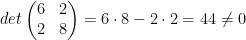
Consider an  matrix , which represents a transformation from
  to
to  . The null space of , written
  is the set of all
  such that
  . The row space of is the set of all linear combinations of the rows of .
To understand why these two sets are orthogonal to each other, let’s write out matrix multiplication in a way that makes it easier to see. We’ll do this with an example of  matrix, but the idea extends to a matrix with any dimensions.
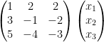 .
.
We would normally understand this matrix vector multiplication as a weighted sum of the columns, or 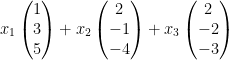 , but we are going to look at it a different way.
Then, we can rewrite as  .
.
We can see that these two ways of multiplying matrices are the same because, for example, the first component of the final vector we just output is 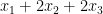 . And if you multiply the ‘s through in the first definition of matrix multiplication above, you’ll get the same thing for the first component of the vector.
Now, let’s consider the vector  . Then,
  . Since
  is in the null space of
  , it must be orthogonal to each row that matrix.
Now, all we need to show is that if a vector is orthogonal to each row, then it is orthogonal to any linear combination of those rows.
Suppose  is orthogonal to every vector in the set
  . Then, let’s compute
  (the right side of the dot is any vector in the span of the
  s). We can rewrite this as
  . We know that
  for
for  , so this dot product is zero.
Thus, is orthogonal to any vector in the row space, and not just each vector that spans the row space.
Overall, we showed that if  , then
  .
.
In the next post, we’ll connect this back to the Rank-Nullity theorem by talking about how the row space and column space of a matrix relate to each other.


 cup of my sourdough starter, and mix that with 113 g fresh flour and 113 g of fresh water. So, even though you discard some starter every time you feed it, you’re always building on the work that you’ve done before. I’ve seen different ratios that can be used to feed a sourdough starter, so I don’t really know how important the exact ratio is. You’ll notice that after feeding your sourdough starter, the yeast really start to produce a lot of
  and the starter gains a lot in volume. So fun!
  to the null space of a matrix. A critical point of a function is a place where all partial derivatives of that function are equal to zero. All polynomials like this are of the form
  , where
  . As a reminder, the null space of a matrix
  .
. . To do this, we will find all partial derivatives of
  . First, we see that
  and
and  . So, to find the critical points of
  and
and  .
.  .
.  , so the Invertible Matrix Theorem tell us that the only vector that solves this equation is
  .
. .
.  . The partial derivatives of
  and
and  . This means we want to solve
  and
and  .
.  , which, by the Invertible Matrix Theorem, means that this matrix equation has infinitely many solutions.
 , which all make
  that takes the value
  and takes the value
  with probability
  .
.  . For a discrete random variable, the expected value is really a weighted average of the possible values of the random variable (weighted by the probability of occurring).
  . Once you know how to calculate this, you might ask what happens if you transform the values that
  , or in general,
  for some
  . For any value of
  , these are called “moments of a distribution,” and they tell you about properties of the distribution.
 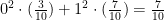 . In this case, since the possible values of the random variable were
  in this case, but that won’t always be true.
  , where
  is the standard deviation of
  to both sides, we get that
  .
.  .
. be a moment generating function for
  and
and  . That’s kind of fun!
  . This was kind of cool because for me, it’s hard to have a geometric understanding of the row space of matrix based on how matrix multiplication is usually defined (
 is kind of hard to picture) but it’s not that hard for me to have a geometric understanding of the null space of a matrix. The fact that they are orthogonal means that if you can understand what it means to be in the null space, then to be in the row space just means that you are orthogonal to everything in the null space.
  .
.  . This should seem really surprising at first. The row space of
  . This represents a transformation from
  , and every output is of the form
 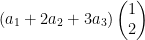 , where
  dimensional (since there’s only one vector that spans the output).
  . This represents a transformation from
  , where
  represents any real number. In this case, the output lives in
  don’t map into the same dimension, the same number of vectors can still be used to represent their outputs! That’s so cool!
  . This has a nice geometric interpretation since any deficiency in the size of the row space is made up for by the size of the null space. It’s amazing how nicely they work together.
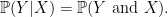
 means “the probability of Y given X.” This comes up a lot when you want to know how the probability of an event changes given that you know whether something already happened. An example of this would be “the probability that I get at A in the class given that I got an 87 on the midterm.”
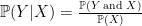 ,
, axes respectively. One way to think about this is that you are trying to find an equation that uses heights to predict weights. Said a different way, you are trying to maximize
  , then it has a null space of dimension
  .
.  has a
has a  . This also means that we can write
  since multiplying a matrix by a vector is just taking a weighted sum of the columns of the matrix. Then you can just move one vector to the other side of the equals sign.
 .
. evaluated at the upper bound of the integral, or
  , or
, or ![[a,b]](https://s0.wp.com/latex.php?latex=%5Ba%2Cb%5D&bg=ffffff&fg=000000&s=0&c=20201002) , you just have to compute the difference in the function’s values at those two points. This makes sense because if someone asks what the total effect of the slope of a mountain was in a region, you would just tell them how high you climbed in that region, or the difference between the height of where you ended and where you started.
, you just have to compute the difference in the function’s values at those two points. This makes sense because if someone asks what the total effect of the slope of a mountain was in a region, you would just tell them how high you climbed in that region, or the difference between the height of where you ended and where you started. 

 (each letter corresponds to a different twist of the cube, and the prime symbol means turn it the way that’s not implied). Whereas before, each edge of the graph corresponded to a single twist of the cube, now each edge represents multiple twists. But, here’s the crazy thing…this graph will still have loops in it no matter what finite set of moves you repeat! It has to, since the graph has finitely many edges!