In this post, I want to talk about the connection between the Rank-Nullity Theorem from Linear Algebra and the First Isomorphism Theorem, which comes up in Abstract Algebra. We talked about the Rank-Nullity Theorem in the last post, but here’s a quick overview.
The Rank-Nullity theorem relates the dimension of the column space of an  matrix
  to the dimension of the null space of that matrix. Specifically, it says that the sum of these two values is equal to the number of columns of . That is,
 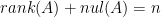 .
.
Before we talk about the First Isomorphism Theorem and relate it to linear transformations, let’s just define a few things that we’ll need to know to understand it.
Definition 1: The kernel of a transformation  is the set
  . Note that
  .
.
Note that the kernel is a generalization of the null space of a matrix that is defined for both linear and nonlinear transformations.
Definition 2: An element  is in the image of a transformation if there exists some
  such that
  .
.
The image of a transformation is a generalization of the column space that holds for both linear and nonlinear transformations. That is, the image of matrix transformation is the column space of that matrix.
Definition 3: A group homomorphism from  to
to  is a function
  such that for all
  and
and  in
in  , it holds that
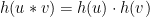
A good way to think about a group homomorphism is that it’s a transformation between groups that maintains the relationship between the groups elements. You will get the same result if you multiply two elements in and apply the function  as if you apply the function to them both separately and then multiply the two outputs in the group
  together. This is interesting because the group composition rules are not necessarily the same.
Now, let’s state the specific case of First Isomorphism Theorem we’ll talk about.
First Isomorphism Theorem: Let  be a surjective homomorphism. Then, is isomorphic to
  . Since
  is surjective,
  .
.
Hold on…What’s does mean? That notation is a quotient group. There is a formal definition of it, but for now, let’s think about it as a way to separate elements in into classes (called cosets) depending on their relationship with  . This quotient group will have two cosets: one containing everything in that IS IN and one containing everything in that IS NOT IN .
Because of the way quotient groups work, if goes between spaces of the same dimension, the original group can be written as the union of two sets: 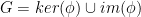 .
.
Since can be written in this way, it must be true that the size of is equal to the sum of the sizes of and  .
.
What does this say about linear transformations represented by square matrices? Since you can’t both be in a set AND not be in a set, it says that for a linear transformation from  to , the null space and column space must be disjoint (except they’ll both have the zero vector in them).
Let’s look at a few examples and see why this makes sense.
Example: Let  be an
be an  invertible matrix. This means that the columns map onto and also that the null space has only the zero vector, meaning that these two sets share only the zero vector.
Example: Consider the non-invertible matrix  , which has the vector
  in its null space. If you try to solve
  , you won’t be able to!
So, what have we learned? The First Isomorphism Theorem generalizes the Rank-Nullity Theorem in a way that lets us handle transformations between groups that are not necessarily Euclidean spaces. There is a tradeoff between having elements in the kernel of a transformation and elements in the image of a transformation. The larger the kernel is, the smaller the image is, and vice versa.
Let’s talk about the progression of these three theorems. The Invertible Matrix Theorem draws connections between the algebraic properties of a square matrix to the geometry of the transformation it represents. The Rank-Nullity theorem makes claims about the geometry of transformations between Euclidean spaces with potentially different dimensions. And the First Isomorphism Theorem makes claims about transformations between groups in general (note that and  are groups for any integers
  and
and  ).
).
In the next post, we’ll talk more about what the First Isomorphism Theorem is actually saying and a neat application of it to transformations between different dimensions.
Stay tuned!


![(A[:,i],A\vec{x}-\vec{b}) = 0.](https://s0.wp.com/latex.php?latex=%28A%5B%3A%2Ci%5D%2CA%5Cvec%7Bx%7D-%5Cvec%7Bb%7D%29+%3D+0.&bg=ffffff&fg=000000&s=0&c=20201002)


![(A\vec{x}-\vec{b},A[:,i]) = 0.](https://s0.wp.com/latex.php?latex=%28A%5Cvec%7Bx%7D-%5Cvec%7Bb%7D%2CA%5B%3A%2Ci%5D%29+%3D+0.&bg=ffffff&fg=000000&s=0&c=20201002)


