Connection between the Normal Equations and Weak Solutions

I want to connect the normal equations, which come up in statistics, to weak solutions, which come up in PDEs. Let’s start with the normal equations. These arise when you want to solve a linear system $A\vec{x}=\vec{b}$ , where $A$ is $m\times n$ for $m>n$ . When you have more equations than unknowns, the system is called “overdetermined.” If your system has no exact solution (which is frequently the case for overdetermined systems), then the best you can do is minimize $\|A\vec{x}-b\|^2$ . This is done by formulating the normal equations $A^TA\vec{x}=A^T\vec{b}$ and solving for $\vec{x}$ . This approach has a lot of issues, but I just want to use it to show a connection to another area of math.

We can rearrange the normal equations and rewrite them as $A^T(A\vec{x}-\vec{b})=0$ . Since $A\vec{x}=\vec{b}$ was the system we wanted to solve originally, $A\vec{x}-\vec{b}$ is the residual vector, or how far $\vec{x}$ is from solving the system exactly. Since $A^T(A\vec{x}-\vec{b})=0$ , this means that the residual $A\vec{x}-\vec{b}$ is orthogonal to every column of $A$ . If we write this in the language of bilinear forms, we get that $(A[:,i],A\vec{x}-\vec{b}) = 0.$ This bilinear form is symmetric, so we can also write this as $(A\vec{x}-\vec{b},A[:,i]) = 0.$

Now, let’s talk about what a weak solution is. These usually come up when differential equations have solutions that might not be as differentiable as the equation itself requires. The idea behind weak solutions is to remove a bit of the strict requirement that a function be smooth enough, as long as it satisfies the other aspects of the PDE. If you wanted to solve a PDE of the form $\mathcal{L}u=f$ for some differential operator $\mathcal{L}$ , the weak formulation instead seeks to solve $(\mathcal{L}u,v) = (f,v)$ , where $(\cdot,\cdot)$ is a bilinear form and $v$ is a sufficiently smooth test function.

Using properties of bilinear forms, we can rewrite this equation as $(\mathcal{L}u-f,v)=0$ .

If we use the example of the linear system we started with, this says that $(A\vec{x}-\vec{b},\vec{v})=0$ for all vectors $\vec{v}$ . This is sort of a weak formulation of the linear system $A\vec{x}=\vec{b}$ .

This looks identical to the result in the normal equations that $(A\vec{x}-\vec{b},A[:,i]) = 0.$ , except that the normal equations impose that particular vectors, the columns of $A$ must be orthogonal to residual $A\vec{x}-b$ , rather than just a general vector $\vec{v}.$

This means that, in some ways, you can think of the least squares formulation of an overdetermined linear system as a weak formulation. In PDEs, weak formulations where the test functions are the same as the elements you’re using to approximate your solution (for least squares those are the columns of $A$ ) are called Galerkin finite element methods.

So that means there’s a nice relationship between Galerkin finite element methods and the least square formulation of an overdetermined linear system!

AM-GM Inequality

The Arithmetic Mean – Geometric Mean inequality says that if you have numbers $a_1,\ldots,a_n\geq0,$ then $(a_1\times a_2\times\ldots \times a_n)^{\frac{1}{n}}\leq\frac{1}{n}(a_1+\ldots+a_n)$ . Another way to say this is that, given a set of nonnegative numbers, their geometric mean is always less than or equal to their arithmetic mean.

Before we look at some examples, let’s think about what this means geometrically. If you raise both sides to the $n$ , you get $(a_1\times a_2\times\ldots \times a_n) \leq \left(\frac{a_1+\ldots+a_n}{n}\right)^n$ . You can think of both sides of this as the area of an $n-$ dimensional box. And this statement says that given sides lengths of a fixed sum, to maximize the volume of the box, you should make each side length the same. That side length is $\frac{a_1+\ldots+a_n}{n}$ .

Now let’s look at some examples where we can apply this theorem.

If $A$ is a positive semidefinite matrix (meaning that its eigenvalues $\lambda_1,\ldots,\lambda_n$ are nonnegative), then $(\lambda_1\times\ldots\times\lambda_n)^\frac{1}{n}\leq \frac{\lambda_1+\ldots+\lambda_n}{n}$ . The product of the eigenvalues of a matrix is $det(A)$ , and sum of the eigenvalues is $tr(A)$ . That means we can write that inequality as $det(A)^{\frac{1}{n}}\leq\left(\frac{tr(A)}{n}\right)$ . We can raise both sides to the $n$ to get a bound on $det(A)$ . We get that, for a positive semidefinite matrix $det(A) \leq \left(\frac{tr(A)}{n}\right)^n$ .

This is nice because the determinant is really expensive to calculate, but the trace is very easy to calculate as the sum of the diagonal entries of $A$ . So this gives an upper bound on $det(A)$ that is easy to obtain.

Let’s consider some positive semidefinite matrices that arise in applications and see what this inequality can tell us.

Let $\vec{f}:\mathbb{R}^n\to\mathbb{R}^n$ be a nonlinear function. Then the Jacobian of this nonlinear transformation is $J=\begin{bmatrix}\frac{\partial f_1}{\partial x_1}&\ldots&\frac{\partial f_1}{\partial x_n}\\ \vdots & \ddots & \vdots \\ \frac{\partial f_n}{\partial x_1}&\ldots&\frac{\partial f_n}{\partial x_n}\end{bmatrix}$ . If the Jacobian matrix is positive semidefinite we can apply the inequality from earlier. It will tell us that $det(J)\leq \left(\frac{tr(J)}{n}\right)^n$ . The right hand side of this can be rewritten as $\left(\frac{\frac{\partial f_1}{\partial x_1}+\ldots+\frac{\partial f_n}{\partial x_n}}{n}\right)^n$ , but this is the same thing as $\left(\frac{div \vec{f}}{n}\right)^n$ , where $div$ is the divergence of a vector field. So we get that $det J \leq \left(\frac {div \vec{f}}{n}\right)^n$ . This is interesting because the determinant of a linear transformation essentially tells you the volume that its basis vectors occupy, and this inequality says that this quantity is bounded above by a function of $div f$ . $div f$ tells you whether $f$ behaves like a source or a sink at a point, so this inequality relates the volume occupied by the linearization of $f$ to extent to which $f$ behaves like a source or a sink at a point.

Now, suppose $g:\mathbb{R}^n\to \mathbb{R}$ is a convex function. Then the Hessian matrix $H$ is given by $H=\begin{bmatrix}\frac{\partial^2f}{\partial x_1^2}&\frac{\partial^2 f}{\partial x_1\partial x_2}&\ldots&\frac{\partial^2 f}{\partial x_1\partial x_n}\\ \frac{\partial^2 f}{\partial x_2\partial x_1}&\frac{\partial^2f}{\partial x_2^2}&\ldots&\frac{\partial^2 f}{\partial x_2\partial x_n}\\ \vdots & \vdots & \ddots&\vdots\\ \frac{\partial^2 f}{\partial x_n\partial x_1}&\frac{\partial^2 f}{\partial x_n\partial x_2}&\ldots&\frac{\partial^2 f}{\partial x_n^2}\end{bmatrix}$ is positive semidefinite. Therefore $det(H)\leq \left(\frac{tr(H)}{n}\right)^n$ . Like in the previous example, we can simplify the numerator. The trace of $H$ is $\frac{\partial^2 f}{\partial x_1^2}+\ldots+\frac{\partial^2 f}{\partial x_n^2}$ , but this is just $\Delta f$ , the Laplacian of $f$ . So this shows that for a convex function (Hessian is positive semidefinite) with Hessian matrix $H$ , $det(H)\leq(\frac{\Delta f}{n})^n$ . If you compute $det H$ at a critical point of the function $f$ (a place where $\nabla f=\vec{0}$ ), you get the Gaussian curvature of the function at that point. That means that this inequality gives an upper bound on the Gaussian curvature at a critical point in terms of $\Delta f$ .

Hopefully this gives some insight into how the Arithmetic Mean – Geometric Mean Inequality comes up in different areas of math!

Why use percent change when you could use logarithms?

Alright, let’s talk about a better way of measuring how something has changed than just using percentages. When you first learn about percentages, they seem like a pretty nice way to measure how things change. Let’s say something increases in price from $10 to $15, you would say that it has increased in price by 50%. Or if something decreases in price from $30 to 20$, you would say that it has decreased in price by about 33%. So, what’s so bad about this way of quantifying things?

Well, consider a different example. Let’s say something costs $50 and then increases in price to $60. We can calculate how much it’s increased in price by calculating $\frac{60-50}{50}=20\%.$ Now, let’s say something costs $60 and then decreases in price to $50. We can calculate how much it’s decreased in price by calculating $\frac{60-50}{60}\approx 16\%$ . This should annoy you! Be annoyed. There’s an asymmetry here. When something increases by $20\%$ , in order for it to get back to its original value, it has to decrease by $16\%$ .

What if we could fix this? What if we could find a way to describe how much something has increased so that when you apply that same description to how something decreased you got a number that was related? What a nice world that would be!

Well…if we use logarithms, we can make this symmetric! Let’s go back to our most recent example. Suppose something increases in price from $50 to $60. Then we can describe this change using logarithms by saying that it increased by $\log(\frac{60}{50})\approx 0.1823$ logarithm points. Now, if something decreases from $60 to $50, we can say that it changed in price by $\log(\frac{50}{60})\approx -0.1823$ , or decreased by $0.1823$ logarithm points. Now these two changes are described in a symmetric way!

Another nice feature of using logarithms to describe changing values is that it makes successive change easier to describe as well. Here’s an example. Let’s say something increases from $5 to $6 and then from $6 to $7. You $\textit{could}$ say that it increased 20% and then 16.7%, but that doesn’t really give you an intuition about the total change. A better way to do this would be to say that it increased $log(\frac{6}{5})+log(\frac{7}{6})=log(6)-log(5)+log(7)-log(6)$ logarithm points. Then some cancellation happens, and we can see that the increased overall $log(\frac{7}{5})$ logarithm points.

I hope this showed you why logarithms can be useful when you want to quantify how much things have changed, and also gave a more intuitive way to think about percent changes that’s symmetric for increasing and decreasing values!

Tell your friends about it! If no friends are nearby, tell a stranger! Make a friend!

Logistic Regression and the Normal Distribution

In this post, we’re going to talk about logistic regression and how it connects to normal distributions. Normal distributions (or scaled/squished normal distributions) come up so frequently in statistics, but sometimes they’re kind of hidden in a problem and it’s hard to tell that they’re actually there. But we are going to find one.

We’re going to talk about logistic regression with a single independent variable and two possible outcomes because that’s easiest to visualize. The goal of logistic regression is to predict which of two outcomes is more likely given some piece of information about the independent variable.

Our running example will be that we want to predict whether someone is male or female based on their height. To do this, we’ll start by plotting peoples heights on the $x-$ axis and whether someone is male or female on the $y-$ axis. Males will be represented as $1$ and females will be represented as $0$ .

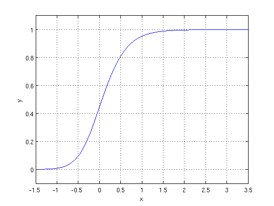
We’d like to figure out a way to guess if someone is a male or female based on their height. We do this by fitting a curve that estimates the probability that a person is male given their height. That will be a curve that looks like something like this:

Image result for logistic curve — (https://en.wikipedia.org/wiki/Generalised_logistic_function)

The place where the two populations overlap most corresponds to the region of the plot near $y=0.5$ . The place where there are a lot of males and females of similar heights means that it would be hard to guess if someone is a male or female just by looking at their height.

The idea is that when a new person comes along, you can look up their height on the $x-$ axis and determine the probability that they are male on the y-axis.

Now let’s talk about how this connects to the normal distribution. The logistic curve that we’re referencing gives us a way of estimating $P(male | height)$ . That is, the probability that someone is male given that they are a certain height.

THE PROBABILITY BELLS ARE SOUNDING. We’re talking about a function whose $y-$ value is the probability that a random variable takes on a particular value. That’s a cumulative density function (CDF)!

To figure out what what probability distribution function (PDF) this is the CDF for, we have to take the derivative of the CDF. That’s because for probability distributions with a single independent variable, the derivative of the CDF is the PDF.

That means we want to take the derivative of the logistic function to figure out the distribution (PDF) that this data came from. That function is the normal distribution!

That means that whenever you perform logistic regression with a single independent variable, you’re assuming that the dependent variable (heights in our case) were normally distributed!

After fitting a logistic regression model to our height data, we could decide some height cutoff (it turns out to be the average height), below which anyone with that height would be classified as female and above which anyone with that height would be classified as male.

What’s interesting is that this logistic regression model corresponds to a normal distribution of heights with the same cutoff.

So anyone with height below 66.368 inches would be classified as female, and anyone with height above 66.368 would be classified as male!

I just think it’s neat that the normal distribution comes up in this way!

Infinitely Long Multiple Choice Tests and Your Old Pal e!

Let’s make up a very ridiculous multiple choice exam and try to figure out how likely it is that you’ll get every question wrong on it. Instead of just thinking about one exam, we’re going to think about a sequence of exams (already sounds like a nightmare, but let’s keep going!), where the $n^{th}$ exam has $n$ questions with $n$ answer choices. So the tests get progressively longer, and each question has more answer choices each time.

If every answer is choice is equally likely and there are $n$ answer choices, then the probability of getting one question right is $\frac{1}{n}$ , and the probability of getting that question wrong is $\frac{n-1}{n}$ . We can also write that as $1-\frac{1}{n}$ . So, the chances of getting every question wrong is $(1-\frac{1}{n})^n$ . Since we care about what happens as the test gets longer and the number of answer choices increases, we want to evaluate $\lim_{n\to \infty}(1-\frac{1}{n})^n$ .

Instead of evaluating this limit, we’re going to evaluate the $\lim_{n\to\infty}(1-\frac{x}{n})^n$ and then set $x$ equal to 1.

We want to evaluate $\lim_{n\to\infty}(1-\frac{x}{n})^n$ , and the first step we’re going to is take the natural log of that expression and exponentiate with $e$ . We can do this since those operations undo each other. So, we want to evaluate $e^{ln(\lim_{n\to\infty}(1-\frac{x}{n})^n)}$ . Let’s bring the $n$ down from the exponent out in front of the logarithm and bring the limit inside of the logarithm to get $e^{n\cdot ln \lim_{n\to\infty}(1-\frac{x}{n})}$ .

Now we’ll just start writing the exponent because that’s the part we’re going to manipulate. If we try to evaluate $ln \lim_{n\to\infty}n\cdot(1-\frac{x}{n})$ directly it won’t really work. So we’re going to rewrite this as $\lim_{n\to\infty}\frac{ln(1-\frac{x}{n})}{1/n}$ . If we try to let $n$ approach infinity, we’ll get an expression with indeterminate form, so we’re going to use L’Hôpital’s rule. That means we’ll take the derivative of the top and the bottom of the fraction separately, and THEN see if we can evaluate the limit. Since we’ll eventually be setting $x$ equal to 1, we’ll treat the $n$ in this expression as the variable and the $x$ as the constant.

Let’s do it. For the numerator, $\frac{d}{dn}\left(ln(1-\frac{x}{n})\right)=\frac{1}{1-\frac{x}{n}}\cdot\frac{x}{n^2}$ . And for the denominator, $\frac{d}{dn}\left(\frac{1}{n}\right)=-\frac{1}{n^2}$ . Now we can get the limit of the original expression by taking $\frac{\text{numerator}}{\text{denominator}}$ .

When we do that, and cross out terms that cancel in the numerator and denominator, we get $-\frac{x}{1-\frac{x}{n}}$ .

So, if we evaluate the original limit we were trying to evaluate, we get $\lim_{n\to\infty}e^{-\frac{x}{1-\frac{x}{n}}}$ . As $n$ approaches infinity, the second term in the denominator goes to zero. so that whole fraction approaches $-x$ .

That means that the limit of the original expression is $e^{-x}$ . When we set $x$ equal to $1$ , this expression evaluates to $e^{-1}$ , or $\frac{1}{e}\approx 0.37$ . That’s the chance of getting every question wrong on a tests of increasing length and number of answer choices.

That means there’s roughly a $63\%$ chance that you’ll get at least one question right! That’s pretty high, considering these this would be for tests with a lot of answer choices.

One way to understand why this is so high is because even though there are more answer choices as you go along in the sequence of tests, there are also more questions, which increases your chance of getting one of them right!

I just think it’s cool that the number $e$ pops up in a probability question like this! I hope you do too!

Six Degrees of Separation

This is building off of the post where I talked about how any two majorities in a set must overlap by at least one element. This is because if you break up a group into a majority and minority and try to make a majority with the minority group, you won’t be able to. You’ll have to take at least one element from the majority group. We’re going to use this fact to talk about how people are connected in social networks. In particular, I want to talk about what kinds of assumptions we need to make in order to find the farthest distance between two people. Distance between people is measured by the number of people you have to go through to be connected to them.

Example: If I know my brother, and he knows his boss, then I’m 1 degree separated from his boss.

Let’s start by laying out the main assumption that we’re making in this problem. We’re going to assume that each person knows the same number of people (which is obviously untrue, but is a reasonable assumption to make). We’ll call this number $n$ . We’ll represent friendships with a graph, where two people are nodes, and a friendship between them is represented by an edge. Since everyone has the same number of friends, every node should have the same number of edges coming out of it. Here’s a sample of what a graph like this would look like.

Note that each node has three total edges coming out of it (except for the bottom layer). Our goal is figure out a general formula for the total number of nodes in this graph, which represents the total number of people accounted for by this graph.

The first layer adds the number of friends that each person has, which is $n$ , or 3 in this case. In the next layer, we add 6 people, which is $(n)(n-1)$ . After a little bit of playing around with sums, you can find that the total of number of nodes in this graph is equal to $1+\sum_{k=1}^{l+1} n(n-1)^{k-1}$ , where $l$ is the number of layers of the graph – 1.

So now, we can imagine somebody else building a network like this one with their friends. We want to figure out when each network will have enough people in it (more than half of the total population) so that we can guarantee that they overlap by at least one person.

In particular, we’d like to find the smallest value of $l$ such that $1+\sum_{k=1}^{l+1} n(n-1)^{k-1}>\frac{N}{2}$ , where $N$ is the total population size.

Here’s an example. Consider a group of 2000 people, where you assume everyone knows 10 people. We want to find the smallest value of $l$ such that $1+\sum_{k=1}^{l+1} n(n-1)^{k-1}>\frac{N}{2}$ . Plugging in these particular values, we want to find the smallest $l$ such that $1+\sum_{k=1}^{l+1} 10(10-1)^{k-1}>\frac{2000}{2}$ , or $1+\sum_{k=1}^{l+1} 10(9)^{k-1}>1000$ . The smallest such $l$ for which this is true is $l=3$ . That means that once we get to the fourth layer of this graph ( $l=$ number of layers $- 1$ ), the total number of nodes accounts for more than half of the population.

Now we can imagine this same process happening for anyone else in the population who’s not accounted for in this graph, and it would also take 4 layers to reach more than half of the population.

Since any two majorities in a set overlap by at least one element, the fourth layer of both sets must share at least one element (person)! That means that we can use that common person to connect both of these graphs. So the maximum distance between the two roots of each graph is $2\cdot$ (depth of each graph) $-1$ , or 7 in this case!

The reason that is so cool is because by just making a few assumptions about how many people are in a population and how many people each person knows, you can figure out the most number of people you’d have to go through in order to connect any two people. What’s amazing about this is that the assumptions you make are pretty reasonable, but the conclusion that you can draw is pretty powerful!

You can do the same thing, but instead think about the population of the whole world and then make assumptions about how many people most people know (this might be how people came up with the 6 degrees of separation idea)!

Why Chickpeas are Cool

I just want to bring this to your attention because it’s so crazy! Whenever you open a can of chickpeas, you probably throw away the liquid that they come in. No longer! That liquid can be used as a substitute for egg whites in baked goods!

In desserts known for their lightness and fluffiness, this is often due to whipped egg whites. Whisking egg whites with an electric beater (or by hand if you’re feeling bold) incorporates air into them and totally changes their texture. When you put the whisk in the mixture and pull out the whisk, if the peak on the tip of the whisk stands up straight without flopping over, that’s called a stiff peak. If it flops over, that’s called a soft peak.

The process of incorporating air into egg whites is the action that contributes most to a meringue’s consistency. It turns out that you can pretty seamlessly replace egg whites beaten to stiff peaks with chickpea liquid beaten to stiff peaks. Just look up the conversion of number of egg whites to number of ounces of egg whites (that can be done on WolframAlpha) and use the chickpea liquid just as you would egg whites! Here’s what the liquid from a can of chickpeas looks like after it’s been whipped for awhile. So frothy!

I just made a pavolva (a baked meringue), following this recipe, https://www.allrecipes.com/recipe/12126/easy-pavlova/ (but replacing the egg whites with the appropriate amount of chickpea liquid, which came out to 4.3 oz of chickpea liquid) and here’s how it came out!

Truly delicious with no evidence of chickpeas!

Determinants and Areas

Let’s prove that the determinant of a $2\times 2$ matrix is the area of the parallelogram spanned by it’s column vectors! Here’s a picture of what that means.

Here are two vectors in $\mathbb{R}^2$ , and a matrix with those vectors as columns. The determinant of this $2\times 2$ matrix is $ad-bc$ . Next let’s look at the parallelogram associated with these two vectors.

To build this parallelogram, you put another copy of the vector $\begin{pmatrix}b\\d\end{pmatrix}$ that starts at the head of the vector $\begin{pmatrix}a\\c\end{pmatrix}$ and you put another copy of the vector $\begin{pmatrix}a\\c\end{pmatrix}$ that starts at the head of the vector $\begin{pmatrix}b\\d\end{pmatrix}$ . Any two non-adjacent sides in this picture are parallel (even though my drawing might not make it seem like that).

Here’s that same picture with all of the important segments labelled.

To find the area of the parallelogram, let’s first find the area of the rectangle and then subtract the area of all of the other triangles.

The rectangle has side lengths $a+b$ and $c+d$ , so its area is $(a+b)(c+d)$ . Note that all of the triangles come in pairs. Let’s start by calculating the areas of all of the triangles, and then we’ll subtract this area from the area of the rectangle afterwards. The area of the right triangle with legs of length $b$ and $d$ is $\frac{1}{2}bd$ , and there are two of them, so the total area to subtract away for those triangles is $bd$ . There are 4 right triangles with leg lengths $b$ and $c$ , so the total area that this accounts for is $4\cdot\frac{1}{2}bc=2bc$ . Finally, there are two right triangles with leg lengths $a$ and $c$ , so the total area that this accounts for is $2\cdot\frac{1}{2}ac=ac$ .

So, to find the area of the parallelogram, we can compute $(a+b)(c+d)-bd-2bc-ac$ . If we multiply out the first term, we get $ac+ad+bc+bd$ .

Subtracting the other three terms, we get $ac+ad+bc+bd-bd-2bc-ac = ad-bc$ . That’s what we were trying to get!

Another reason that this is cool is because we can actually think of $ad-bc$ geometrically in a SECOND way also! Not only is it the area of the parallelogram, but it’s ALSO the difference in area of two rectangles: the rectangle with side lengths $a$ and $d$ and the rectangle with side lengths $b$ and $c$ , which are both in that picture! That’s not intuitive at all if you ask me!

How crazy is that?

Sourdough Baking — Day 3

Okay, it’s finally here. The day you get to bake bread. I’d first like to say that I went the entire day without setting the smoke alarm in my apartment off (which happened 3 times the last time I did this), so I’d already consider that a win.

The first thing to do on Day 3 is preheat your dutch oven that you’ll be baking in. Two good things about a dutch oven is that it holds heat really well and the top helps trap steam so that the crust can remain soft for the first few minutes and the dough can continue to expand as it cooks. If you only baked without the top, the outside would finish cooking before the dough expanded to the ideal size and the inside would be gummy.

Preheat the dutch oven with its top on at 500 $^\circ \text{F}$ for 1 hour. If the handle of your dutch oven is plastic, you should unscrew it. Then cut parchment paper to the size of the dutch oven you’re baking in. A good way to do this is to fold a square of parchment paper in quarters, then fold in half to make a triangle, and do this a few times. Then cut a little parchment paper off the top. When you unfold it, you should be left with a circle-ish shape (or a shape with, like, 30 sides). Sift flour onto the parchment paper so the dough doesn’t stick to it.

{Take one loaf out of the fridge. Flip the dough out from the proofing basket onto the floured and beautifully cut parchment paper and score (make cuts in the top of the dough) the dough in a pattern of your choosing. The best tool for this is a lame (French — pronounced like the first syllable of llama). It looks like this.

This helps steam escape from the bread and encourages it to rise. The blade is scary sharp so be careful.

Here’s what the scored dough looks like on the parchment paper.

Take the dutch oven out of the oven. Slide the parchment paper with the dough into the dutch oven and put the cover back on.

Put the dutch oven in the oven and bake for 15 minutes with the lid on. After 15 minutes, take the lid off the dutch oven. Bake for an additional 30-40 minutes. The crust should be firm to the touch (but it should also be really hot, so be careful!). The inside of the dough should register 190 $^\circ \text{F}$ with cooking thermometer (do different thermometers give different temperatures? Probably not. But it should be pointy enough to puncture the outside of the bread). I baked mine for 35 minutes, but all ovens are different, so you should keep an eye on it. You can tap on the bottom of the bread, and if it sounds hollow, it means the bread is done.

[One big inhale…] Take the dutch oven out of the oven and transfer the bread (without the parchment paper) onto a cooling rack. Let the bread cool for a few hours before cutting into. The inside needs time to set to achieve the texture you’re really after!}

Congrats! You just baked a loaf of sourdough bread! Now just repeat everything inside of the {}s for the second loaf. You can experiment with different scoring patterns!

Here are what my loaves looked like today!

I still haven’t quite figured out how to get the sections between the scores to be at different heights (like the inner circle popping up over the outer circle). I think that look cool, but it’s nice to have things to work towards.

I’d like to give an enormous thank you to Brad and Claire at Bon Appetit for the inspiration to do this and for the incredibly helpful video that explained each step of the process!

Sourdough Baking — Day 2

By the next morning, the mixture of flour, water, and starter from the day before should look something like this.

You can see that it’s gained a lot in volume. That’s a good sign because it means the yeast is producing a lot of gas! To tell if the starter has fermented enough overnight, you do something called the float test. Put a small spoonful of the starter into a bowl of water. If the starter floats, then that means it’s fermented enough overnight to continue. Here’s what a successful float test looks like.

In the next step, called autolyse, you mix the remaining flour (1000 g) with a portion of the remaining water. You can let this go anywhere from 30 minutes to 2 hours. Since the starter doesn’t actually get used for another 30 minutes to 2 hours, if your starter didn’t pass the float test the first time, then it should by the time the autolyse is finished.

Here’s how to make the autolyse. Mix 1000 g of flour with 750 g of water until a shaggy mass forms. A wooden spoon works great for this!

I didn’t take a picture of the next step because by the time I thought about it, both of my hands were covered in dough, but here’s what you’re supposed to do (then I’ll tell you what I did, since I messed up a little). Add 200 g of the starter to the autolyse, and pinch in the starter with your thumbs and pointers. While you are doing this, you can be flipping the dough over so that the starter gets fully incorporated. This is also when you can incorporate any remaining dry flour. Next, add 20 g of salt over the dough and pour 50 g of water to dissolve the salt. Pinch again to incorporate the salt, rotating as before.

Here’s what I did accidentally. I forgot to add the water at first, so I just pinched in the 20 g of salt without adding any water. Then I added 50 g of water after pinching in the salt. I mixed the dough with a wooden spoon to make sure the water was all incorporated.

The next step is called slap and fold, which I also didn’t take a picture of because both hands were covered in dough and I have no way to mount my phone. You can look up what that looks like if you want. Essentially, you are picking up the dough and throwing it down on the table. Before you pick it back up, you want to fold the dough over itself so that as you’re throwing it down the next time, it’s kind of in one compact mass. Keep doing this until the dough gains some structure and becomes less slack.

Next, is the “you have to wait just long enough to watch an episode of a show but not long enough to go be productive” step. After slapping and folding, put the dough into a large bowl. Every 30 minutes, give the dough a series of folds. Lift up the dough from the center, and kind of let it fall onto itself. Do this a few times, and then turn the bowl 90 degrees. Do this 6 times (so this step should take 2.5 hours).

In the next step, you divide the dough into two halves using a bench scraper (try to be as precise as possible, but it’s not a huge deal if one piece is slightly bigger than the other). Try to coax the dough into a rough circle, then sprinkle a little flour over the tops of them. Then cover the two masses of dough with a clean towel and let them rest for 10 minutes. You’re doing this because you just stretched the gluten, so you want to give the strands a chance to re-form.

After the dough’s had a chance to rest, you want to flatten it out by tugging on the outer edge of it. Fold the part furthest away from you in towards the center. Then fold the right, then left parts of the dough in towards the center. Then fold the bottom part up. Pinch along the seam you created (called stitching) and flip the dough over seam side down so it seals.

Then place the dough into floured proofing baskets seam side up (the bottom is pointing up), and let rest in the fridge covered with a towel overnight. Mine will end up being in there around 19 hours, so we’ll see how they look when they come out of the oven later. Here’s what mine looked like before I refrigerated them.

That’s the end of day 2! The next day (which is actually today), it’s finally time to bake them!